Representation of the Hi-C World

1. Background

All my PhD work revolves around this data called "Hi-C," which are contact matrices that show where the DNA in the chromosome makes pair-wise contacts, like if you knew the exact 1D indices along a string, you'd measure whereever the string touched another piece of itself. Combine this thinking to millions of cells and pool your results, and you have a Hi-C contact matrix (or also Micro-C or other Chromatin Conformation Contact (3C) Map style data).

A big issue is that studying Hi-C, we often end up with issues of solving for special features. Without getting into too much detail, the most popular feature to study is called the Chromatin loop. Loops are thought to in many cases bring all the gene and binding-site components close in space. On a chromatin contact matrix, they look like wider, higher signal spots, like so.

The problem is most ways to solve loops are threshold based algorithmic callers, which can be well tuned to a reference dataset, but suffer issues with a high rate of false positives. Sometimes as high as 40%

This problem is sidestepped by biologists and bioinformatians who enjoy Hi-C (and Micro-C) by performing aggregate loop pileups, which is called aggregated peak analysis. You take all the windows over the Hi-C loops, you scale them to the same size and normalization per window, then you average everything and visualize the result.

In my mind, this only really makes sense if you have a masterlist of loops, otherwise who knows how much of your data is false positives, to say nothing of the lost true positives due to thresholding in tricky regions of the contact map.

1.1 Image Work

Early in my PhD I struggled with this problem, and I tried a few ways to handle choosing a refined set of chromatin loops. Using sequence data, like certain proteins that bind DNA near where the anchors (or the X,Y coordinates on the contact frequency matrix) is not useful, as many loops seem to be independent of CTCF and RAD21, the canonical binding factors thought to faciliate chromatin loop formation. Besides, most chromatin architectural feature callers for loops, stripes, and topologically associated domains rely on visual cues. So I went through several phases of finding a way to relate chromatin loops in a way that takes advantage of image processing techniques without using outright thresholding.

I had some initial success with subclustering chromatin loops using a naive approach. I normalized submatrices (individual loop windows) and, using sinkhorn estimators, used agglomerative clustering and cut to form groups. The groupings were compelling, but it wasn't enough for a paper. Using agglomerative clustering was also very restrictive, becoming very slow/intractable at massive scale. A few years were spent on Quagga and another applied paper before I returned to the problem. To keep things neat, I'll say here that the correct approach was to force our submarices into 128px images using the same normalization and bilinear interpolation, to use sliding window fast fourier transform with hellinger's distance, and to replace agglomerative clustering with a local k-means on subsets of eight thousand on a 30 million image (submatrix) dataset.

1.2 Hi-C Video Clips

After a whole year of getting back into machine learning, I spent the Fall of 2025 trying various video models. I wrote video shimm, a weird, messy approach to learning video modeling instead of World Model. I had a realization. If my chromatin loops are semantically similar in a visually defined way, and if I make my latent representations of loops not purely reconstructive and somewhat semantic, I may be able to solve my issue of loop false positives learning a representation space and also teaching a latent traversal to effectively flag membership.

I would reuse the clustering strategy I had developed, sampling with random order within the k-means clusters to form hi-C "video clips." This meant using the same ideas in representation learning. I liked this because I was already familiar with checking local lipschitz and token churn in VQ.

With a stable representation in the VAE, the claim I make is that our representation which is focused on image similarity, should allow representations of chromatin loops to lie nearby in our representation manifold.

Once this is shown, we need only use a subset of loops that are annotated before hand and we can solve any random patch given to the model to determine its membership. With the VAE alone we can solve this in continuous or discrete space. Using token mass based on PLL from annotated data is the easy way, and we can apply this to VQVAE. Using cosine distances on Z from something like ß-VAE is more work, but more elegant because we borrow most of the representational abstractions from continuous latents anyway.

Continuous Representations

Even while working with discrete VQ token grids, my intuition about representation space keeps drifting back to a continuous picture. In practice, this mental shortcut often works: combinations of tokens behave as though they lie on an underlying smooth manifold. There’s a certain irony here — the straight-through estimator that lets gradients pass through quantization is mirrored by the way we reason “straight through” the discrete layer when thinking about latent geometry.

In reality, the model never operates directly in a continuous latent space. Encoder outputs (Z_e) are snapped to the nearest codebook entries (Z_q), and downstream models — including transformers operating over tokens — only ever see these discrete symbols. Any continuous interpretation emerges only when we project back into embedding space for decoding. This tension between discrete computation and continuous intuition is exactly what motivates exploring an explicitly smooth latent space.

That, and after maybe 3 weeks of doing it this way and being questioned my friends, family, and my PI if I had bothered to try just simply using the smooth latent space, I ran out of excuses. So here we are.

3. WAN2.2 Variational Autoencoder

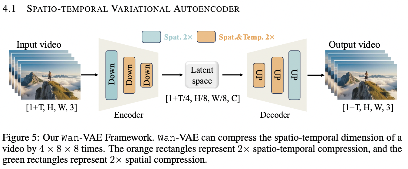
Recently I experimented with switching to a continuous autoencoder, starting with WAN 2.2. Since the training details for WAN 2.2 are not public, I followed the WAN 2.1 VAE training regime on a 5080. WAN's VAE is trained in several distinct phases. The first phase mirrors standard 2D training, except their 3D ConvNet is trained using a single frame sampled from each video clip, treating time as an auxiliary axis rather than a predictive sequence. In the second phase, the ConvNet is inflated to use a sequence of video frames and does causal masking.

WAN Initial Pretrain (2D and 3D):

$$\mathcal{L}_{loss} = 3 * \mathcal{L}_{L1} + 3 * \mathcal{L}_{LPIPS} + 3e^{-6} * \mathcal{L}_{KL}$$

Finally, at the very end, we finetune using adversarial loss. Doing it this way, latent generation is prioritized over detailed perceptual/reconstructive gains.

WAN Adversarial refinement (best guess):

$$\mathcal{L}_{loss} = 3 * \mathcal{L}_{L1} + 1.5 * \mathcal{L}_{LPIPS} + 3e^{-6} * \mathcal{L}_{KL} + \underline{0.5 * \mathcal{L}_{adversarial}}$$

Compare this to Tencent's Hunyuan video model, where the entire 3D SpatioTemporal ConvNet is trained at once using a small adversarial loss from the beginning. The hand-wavy explanation I can offer to this is that reconstruction (and realism, apparently) are more prioritized in Hunyuan over latent generative capability. They also use curriculum dynamically in pretraining over distinct phases, gradually training from low-resolution short video to high-resolution long video, and randomly choose between 1 to 8 frames per video for reconstruction explicitly.

Hunyuan's Pretrain:

$$\mathcal{L}_{loss} = \mathcal{L}_{L1} + 0.1 * \mathcal{L}_{LPIPS} + 0.05 * \mathcal{L}_{adversarial} + 10^{-6} * \mathcal{L}_{KL}$$

I'd point out that they both approach the well known problem that discriminators from GAN can completely overpower the generative power of the VAE. WAN pretrain handles this by doing a very strong train and cleaning up reconstruction detail at the very end, whereas Tencent allows the GAN to run from the beginning, but downweights the effect it has substantially, so that it cannot overpower the learning VAE.

WANVAE Pretrain Phase 1

I walk through recreating WAN2's VAE in the first phase. While Hi-C will require a different set of assumptions, we can try it out in video first.

In the first phase we see about 14,000,000 video frames, which is probably sufficient to probe whether a smooth latent space emerges and to compare its behavior against the VQ-based representation.

The faces look pretty weird. I use VGG style LPIPS for the entire training, which is considered 'richer' than alexnet. I think on paper L1 and LPIPS weighting team WAN uses seems very high at 3.0 and 3.0 at first glance. But, honestly these are just scaling factors, and as long as our metrics for perceptual loss are roughly proportional and slightly below the L1, it's not a big deal. As for the artifacting, the bet is we can ignore reconstruction to learn as good a well-formed manifold as possible before correcting it at the end using adversarial loss with a finetune.

Stopping criteria here is (1) KL loss, L1 loss, and LPIPS loss flatten, (2) the frame-by-frame VAE reconstruction seems to no longer improve nor get worse (stabilization).

WANVAE Pretrain Phase 2

Then we expand the ConvNet to 3D. The reference paper divides the video sequence into 5 "sequence" groups, the first image is set apart, and the remaining frames are split into 4 groups, which form the bulk of the latent. To do this we set our 2D Convnet to fill the structure of the entire 3D structure and simply fill the remaining space with either random or zero. I use zeros.

This also means we'll have to rein in our batches and our latents now represent a temporal block containing 1/5 of the video clip, so motion and dynamics are well captured in the latent. WAN-VAE uses causal masking in it's time dimension. This will be a problem for Hi-C and I'll explain and change it later, but for now just know we pad more of the past to predict the current temporal block t.

What I have here is a clever trick to deal with the assymetric encoding-decoding issue. We encode 5 frames into a latent and this decodes, due to the padding and convolutions to 8 frames. We simply write the video to pad 5 frames to 40 (repeat each frame 8 times) and in the decode repeat each frame 5 times, and use a shared FPS. We also see the same issue of the starting latent frame (leader frame) being degraded as it has less context than the rest of the decoded latent.

We train it much longer as the KL loss continues to drop.

WANVAE Pretrain phase 3

Finally, we introduce detail with adversarial loss.

3.1 WANVAE with Hi-C

The idea ports pretty well into Hi-C. I remove all the RGB channels and set it to a single greyscale channel. I also discard perceptual loss (LPIPS alexnet) and instead use a tiny Structural similarity index measure (SSIM) score. I considered multi-scale SSIM or multiscale-L1, but decided against it.

Something else to consider is we have an image processing and normalization procedure that is outside the typical. Basically we're turning a spectral matrix into an image, and we're using raw matrices with no normalization. Our own normalization is effectively min-max scaling with a specially solved maximum, which can be lower than the true maximum in the image, so we clamp our normalized matrices [0,1]. Because WAN VAE (and many VAEs) use tanh activations and run [-1,1], we need to carefully cast between [0,1] and [-1,1] where appropriate. Not the end of world, just tedious.

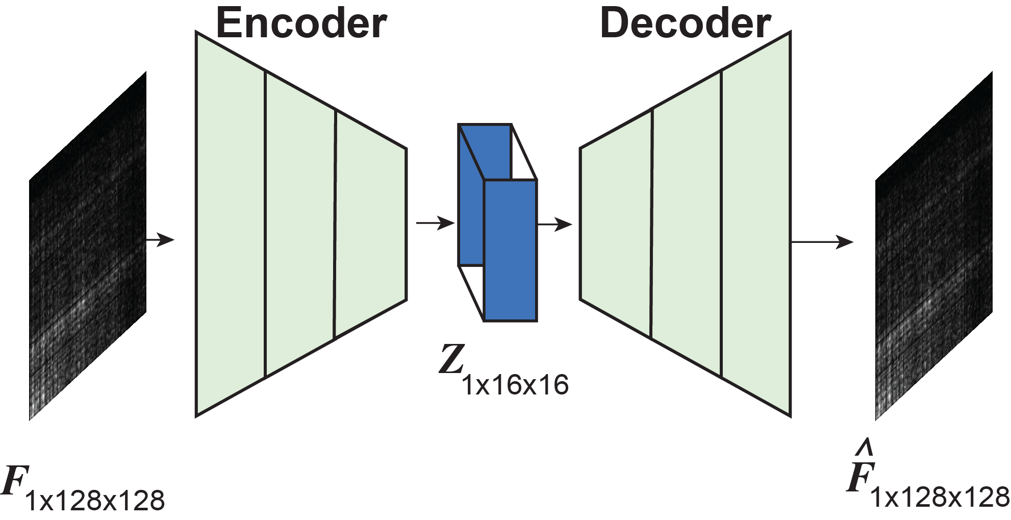
"Video" Hi-C

Unlike with the VQ-VAE, we can easily push the idea of using video to scale out WAN's VAE so long as we have something that resembles a temporal sequence. We effect this with some careful assumptions that we can map sets of our Hi-C image patches into small clusters, using a combination of sliding window FFT, hellinger distances, and overlapping subsets and an 'overflow' queue using k-means.

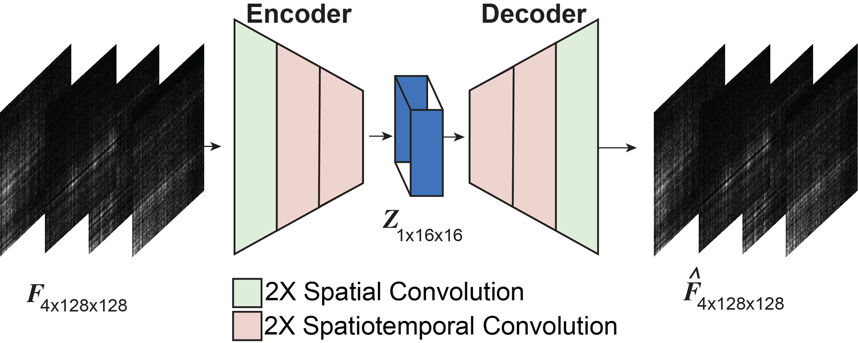
The point of doing this is to steer an inductive bias, where related images are forced together as a latent tensor point, rather than by happenstance. This means we can effectively force points that are tied up in the k-means miniclusters together in latent space, although their interpretability now because deeply entangled.

3DVAE footguns

Standard 3D ConvNets, such as those implemented with torch.nn.Conv3d, treat the temporal axis identically to spatial axes and are not inherently causal. However, many video modeling pipelines impose temporal directionality through asymmetric padding, causal masking, or next-frame prediction objectives.

This means we can't just reuse WAN2-VAE as is, as our "video" isn't really a markov chain, more like a dense subgraph of a larger search surface; we want to claim that a transition between any of the states is fine. So causal masking won't do us any good in attention nor in our ConvNet padding.

Because we model frames whose order doesn’t matter (valid transitions between any of them) we only treat the data like a video for architectural convenience. That means we avoid video style causal masking and instead use symmetric padding along the time axis. With Hi-C 3D latents intended to be time-invariant, treating time like another spatial dimension encourages consistency and smooth transitions rather than next-step prediction.

Many video pipelines introduce temporal directionality via causal padding (e.g., using past frames [t−2, t−1, t]) to support forward-in-time tasks. That’s useful for streaming or prediction, but for representation learning and diffusion it can impose an artificial ordering. Symmetric padding ([t−1, t, t+1]) better matches our goal of a time-agnostic latent structure. Since there is no privileged “future” or “past” in this setting, we’re not concerned about information leakage, only about maintaining coherent structure across frames.

And in WAN2.2 VAE's reference implementation, we change the padding and rename CausalConv3d to SymmetricConv3d for clarity.

We leave the task of predicting "next" or interpolated "t" to DiT if we really want it. This also means instead of inflating from 2D to 3D by placing the learned 2D weights in the current timeslot of the 3D model that is represented by the final padding, we use the center so we obey the symmetry we pad for. Hopefully that's clear. Now, lets get on with it.

WANVAE with Hi-C Pretrain phase 1

Here I'm using dual H100s with a global batch of 600. If we see 14M images in 1M steps with batch 14 on my 5080, two H100s see something similar in 23K steps. You'll notice near 20K steps the reconstructions are not convincing, why? The napkin math isn't a good rule, and there is often diminishing returns for scaling batch size, especially for our VAE which is about 175M parameters. Our dataset is about 28M Hi-C images that form into nearly 7M clips. So we still need to step enough for our model to learn a well behaved latent manifold after phase1. We'll see 60,000,000 individual frames in phase 1.

Stopping criteria is similar to the video implementation, convincing looking VAE decodes, and plateaus in decreasing L1, SSIM, and KL loss.

After 100K steps I'm satisfied. We inflate our model to use its 3D ConvNet behavior with the symmetric padding we implemented.

WANVAE with Hi-C Pretrain phase 2

We expand the 2D ConvNet's final checkpoint like decribed in WAN's implementation report, but for symmetric not casual 3D ConvNets. Using symmetric masks and dropping positional encoding lets us learn time independent frame transitions. The math works out to 12,000,000 T=5 clips seen in our second training phase.

Stopping criteria is the same to the 2D, convincing looking VAE decodes, and plateaus in decreasing L1, SSIM, and KL loss.

After about 200K steps our metrics look OK and the representations are quite stable from a cursory look. So now we'll get into doing a non-heuristic evaluation of our Hi-C WANVAE. Image/Video detail is not important here, so I skip adversarial loss entirely. We're ready to start analyzing our representational manifold and how well it behaves. If it's well formed and locally euclidean, we can use it for direct interpolation.

WANVAE with Hi-C Pretrain phase 3

For completeness, we use adversarial loss to introduce more detail in the decode process. Stopping criteria is the same to the 2D, convincing looking VAE decodes, and plateaus in decreasing L1, SSIM, and KL loss.

It looks alot more convincing, but not perfect. Some artifacts are introduced that look like specs of dust. But the GAN finetune is mostly a decoder beautification, and doesn't affect our representation geometry.

3.2 Scoring Continuous Representational Space

As with VQ-style representations, we can ask whether our latent space behaves “well,” but in the continuous case this means something slightly different. A well-behaved latent manifold is locally Euclidean: if you zoom in far enough, curved structure looks linear, much like approximating a small segment of a 2D curve with its tangent. In high-dimensional latent space, this corresponds to local Lipschitz continuity with a constant near 1, ensuring that small moves in latent space produce proportional changes after decoding. When this holds, linear paths map to smooth transitions, nearest neighbors are semantically similar, distances become meaningful for search and clustering, and small perturbations do not destroy structure.

This differs from the VQ setting, where the latent space is discrete and “good behavior” is piecewise smooth: nearby inputs should map to the same or neighboring codes, quantization error should remain low, and transitions between codes should be semantically coherent. In the continuous case, mixtures always remain on the manifold by construction; the question becomes how well our inductive biases and reconstruction objective shape a geometry that preserves similarity without explicit supervision.

If we succeeded, interpolating between two states within the same clip should produce reasonable intermediate states. If we fail, interpolation will reveal geometric pathologies: abrupt transitions, implausible structure, or artifacts that were absent in both endpoints. In video this appears as teleporting objects or discontinuous motion; in Hi-C it may manifest as identity diagonals, loops, or voids emerging in the interpolation despite being absent in both the source and target frames.

Geometric intuition for local linearity

Suppose we have a function or neural network that learns a manifold embedded in $\mathbb{R}^d.$ For intuition, we illustrate the geometry with a toy example in $\mathbb{R}^2$, where the learned representation lies along a 1D embedded manifold. This is a simplified visualization of the more general case in which a lower-dimensional manifold is realized within a $\mathbb{R}^d$ bottleneck. The figure below shows a good manifold ($M_a$), an okay one ($M_b$), and a poor one ($M_c$).

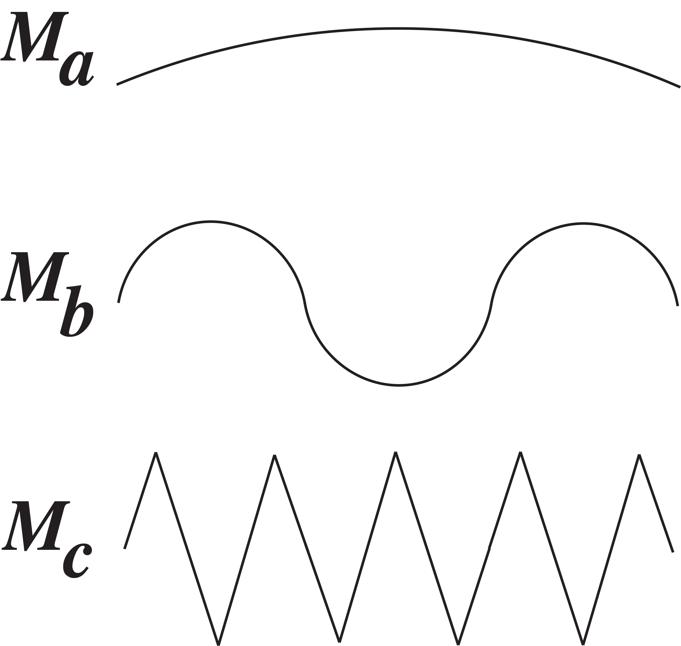
Imagine all the points in our representation could be embodied by one of these three surfaces.

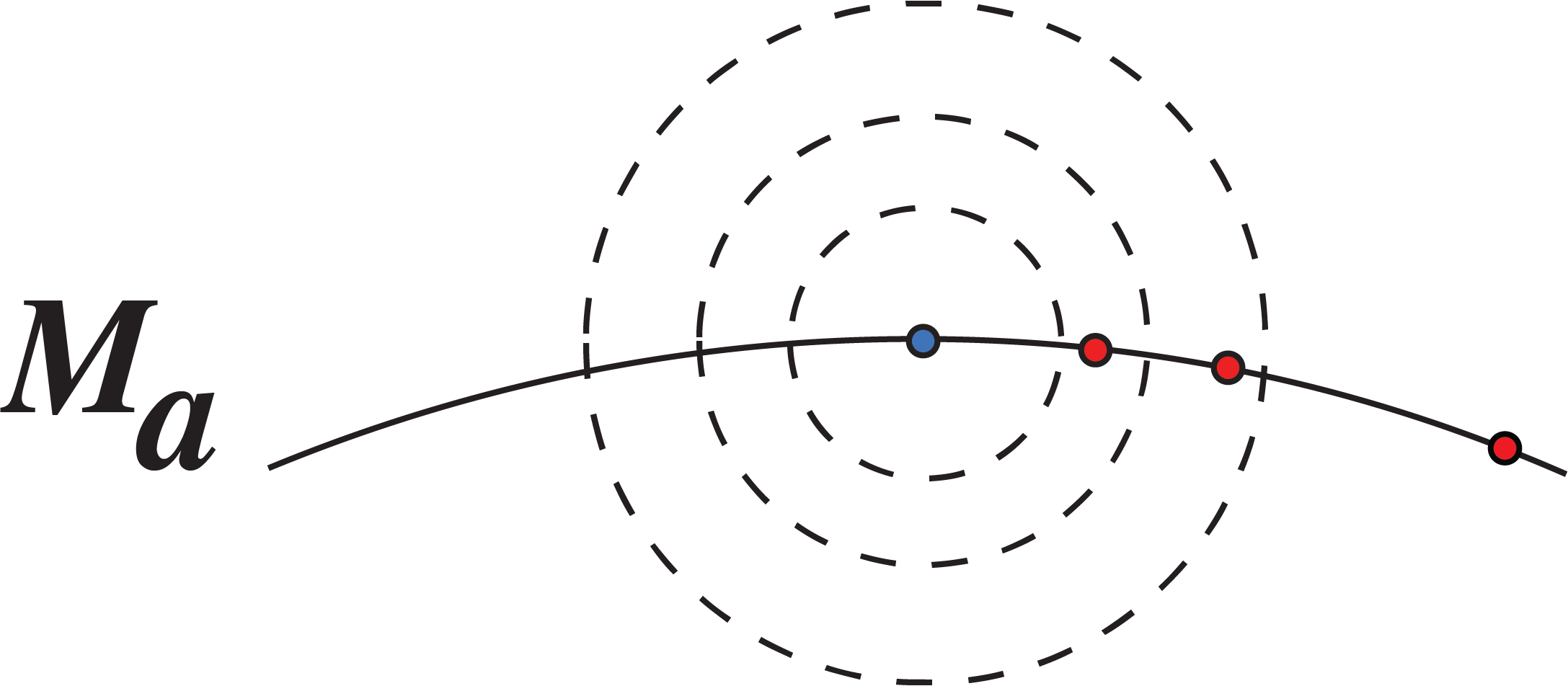
In the first case, $M_a$, the manifold is gently curved. Metric distances are well behaved, and within a sufficiently small neighborhood the straight-line distance between two points becomes a good approximation to the nonlinear distance along the surface itself. This local Euclidean property is exactly what makes latent interpolation, nearest-neighbor search, and membership reasoning plausible.

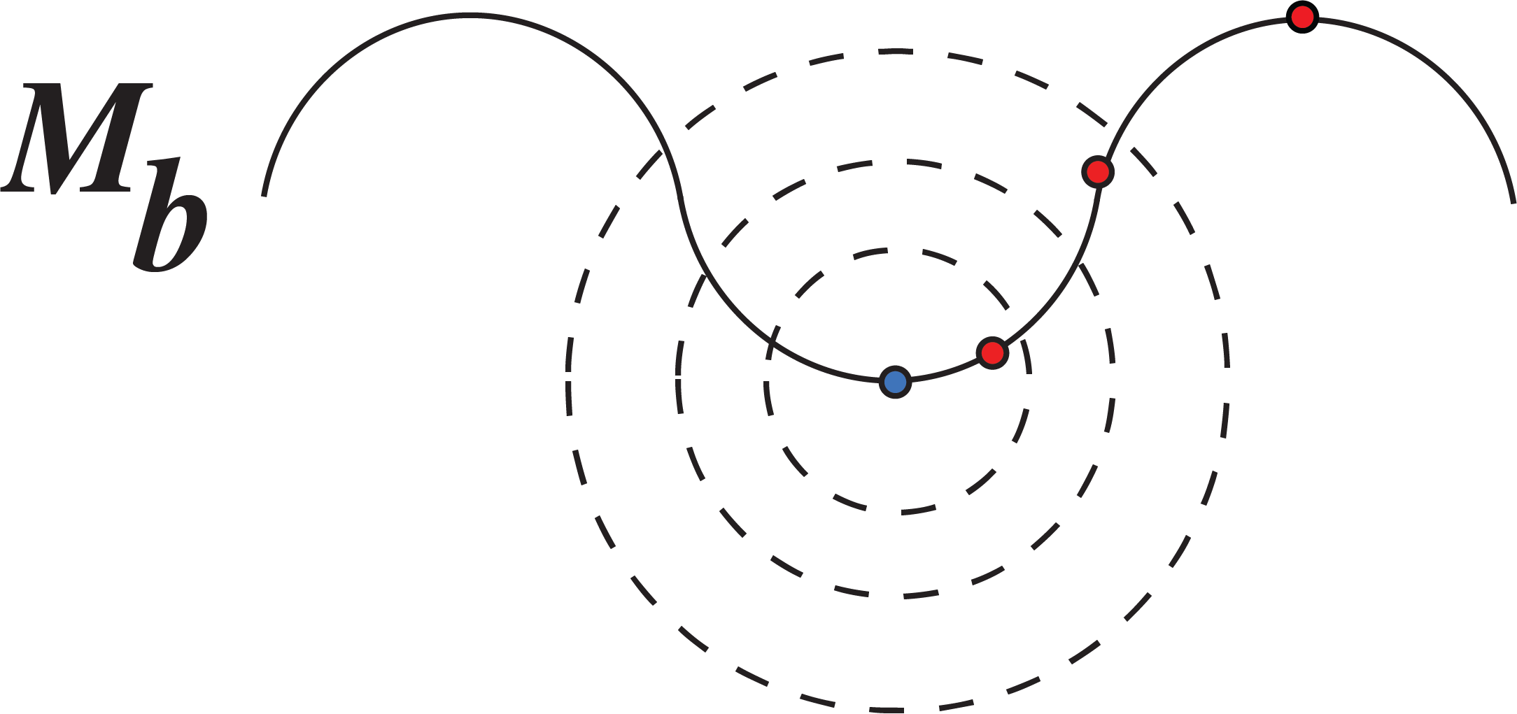
In the second case, $M_b$, the metric is still useful, but only if we restrict ourselves to a smaller radius. Distances behave sensibly only below some local $\varepsilon$ scale. With that caveat, interpolation and local search can still work.

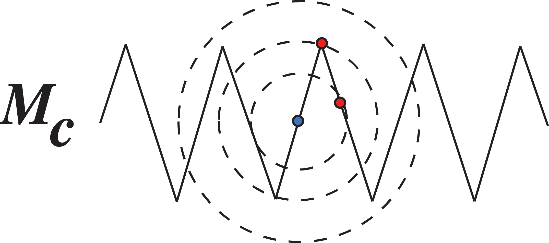
In the third case, $M_c$, the manifold is too jagged or folded. Distances in the ambient space no longer reflect meaningful distances along the manifold, so interpolation and kNN-based reasoning become unreliable. This is the failure mode I want to rule out empirically.

I want my latent manifold to behave euclidean locally like the first or second case. I do not want it to act like the third. For the sake of sanity, you can often 'get away' with training a good model without explicitly using second order regularization (like lipschitz regularization), or the VAE and beta-VAE researchers like to enforce a global euclidean distribution to match their Gaussian Prior. How can I claim this? I check the manifold empirically.

Same-vs-other separation

The first thing I want to know is whether annotated loop clips and non-loop clips are even separable in latent space before I start making stronger geometric claims. So I encode all labeled clips to their posterior means, flatten the latent, and compare pairwise scores between samples from the same class against samples from different classes. For cosine-family metrics, larger means closer; for L2, smaller means closer.

$$\mathrm{AUC}_{\text{same} > \text{other}} = \mathbb{P}\Big( s(z_i,z_j) > s(z_i,z_k) \;\big|\; y_i = y_j,\; y_i \neq y_k \Big)$$ $$\text{or for } L_2:\qquad \mathbb{P}\Big( d(z_i,z_j) < d(z_i,z_k) \;\big|\; y_i = y_j,\; y_i \neq y_k \Big)$$

This is an intentionally simple ranking-style readout: if the manifold is doing anything useful, a random same-class pair should beat a random cross-class pair more often than chance. I also track the latent norm distribution by class, because a degenerate model can appear separable only because one class is systematically assigned larger or smaller latent magnitude.

Local neighborhood membership

Pairwise separation is useful, but it does not tell us whether the local neighborhoods of the manifold are coherent. For that I use k-nearest-neighbor purity and an $\varepsilon$-ball membership analysis over the same latent means.

$$\mathrm{kNN\ purity}(i) = \frac{1}{k} \sum_{j \in \mathcal{N}_k(i)} \mathbf{1}[y_j = y_i]$$ $$\mathrm{lift} = \mathbb{E}[\mathrm{kNN\ purity}] - \sum_c p(c)^2$$

The baseline term $\sum_c p(c)^2$ is the class-prior chance level: it is the expected same-label match rate if neighbors were assigned at random according to class frequency. So positive lift means the latent neighborhoods are more class-consistent than chance, even after accounting for imbalance.

$$\mathrm{margin}(i) = \begin{cases} s\big(z_i, z_{\text{nearest same}}\big) - s\big(z_i, z_{\text{nearest other}}\big), & \text{cosine family} \\ d\big(z_i, z_{\text{nearest other}}\big) - d\big(z_i, z_{\text{nearest same}}\big), & L_2 \end{cases}$$

I also sweep explicit local thresholds. For cosine-family metrics an $\varepsilon$-ball is really a minimum similarity cutoff, while for $L_2$ it is an ordinary radius. At each threshold I record coverage, mean purity on covered samples, and how many same-class versus other-class neighbors fall into that local ball. This gives a direct picture of how stable or contaminated local membership becomes as I widen the neighborhood.

Local decoder geometry

Once a latent can separate classes locally, the next question is whether interpolation and local search are geometrically trustworthy. I probe this with finite differences around encoded data latents rather than with global assumptions about the manifold. These are local decoder-space tests, not a proof that the full latent support is globally Euclidean.

$$J u \approx \frac{D(z + \epsilon u) - D(z - \epsilon u)}{2\epsilon}$$ $$G = (JU)(JU)^\top$$

Using random orthonormal probe directions $u$, I estimate a local singular spectrum of the decoder Jacobian from the Gram matrix above. From that I read off the largest and smallest probed singular values, a local condition number, stable-rank style summaries, and anisotropy surrogates such as how dominant the top singular mode is.

$$\partial_{uu} D(z) \approx \frac{D(z + h u) - 2D(z) + D(z - h u)}{h^2}$$

I then measure second directional differences as a curvature surrogate. Small values mean that in a neighborhood of the current point, the decoder behaves almost linearly along those directions. I report these both in absolute RMS units and relative to the local Jacobian scale, which makes it easier to compare points whose decoder gain differs.

$$\mathrm{gain}(\epsilon, u) = \frac{\lVert D(z + \epsilon u) - D(z) \rVert_{\mathrm{RMS}}}{\epsilon}$$

Finally I look at finite-step gain, which is a practical local Lipschitz test. This complements the infinitesimal Jacobian estimate: even if the Jacobian looks reasonable at one point, a finite step can still reveal nonlinear expansion or collapse.

3.3 Continuous Latent Interpolation

Swapping to a VAE style gives us some new advantages and problems. Problems: (1) we're no longer token native, so we can't just define a context window limit for a GPT2 or BERT and teach it to return frame-sized token grids to decode; (2) token mass tricks and PLL for assigning token alignment towards loops or non-loops won't work here, which is an easy and compelling result. Advantage: (1) we no longer need an engine to perform interpolation, we can do continuous mixing of latents, interpolate directly, or just perform raw search over the latent manifold; (2) diffusion and rectified flows are now much more accessible, although this opens up a new "can of worms."

To explain the problem with using RF/Flow-matching, with GPT2 or BERT, bad dense subgraphs (our video clips) are acceptable as long as they're rare. With OT problems, this causes miscoupling. I can think of some great CS experimentalists when the Drift paper was released who wanted to use Characteristic functions on the latents of JEPA to better do OT couplings. This is something like using the FFT of a PDF of your dataset as the method for doing pair-wise coupling. To really oversimplify this, OT effectively learns a direct map from group A to group B. If you have several distinct classes in group B that can be seen as checkerboards with 4 squares, 16 squares, and 1024 squares, doing histograms, 2DFFT, or characteristic functions are blind to the differences here. In this kind of case I'd point out this is a place where SDE styled diffusion may win out.

Direct interpolation (for the sanity of me, my friends, my family, and my PI) is what I ended up going with.

Image/Video latent interpolation

A brief explanation here will motivate why I'm avoiding doing a KL enforced prior (VAE with beta = 1) and still claiming we can walk the latent surface our Autoencoder forms. The important point is not that the full manifold is globally flat, but that the local neighborhoods are well-behaved enough that linear interpolation between nearby points remains meaningful.

2D/3D Hi-C latent interpolation

3.4 Unconditional Sampling and Generation

Something interesting with Variational Autoencoders is that they're structured with a prior that can be sampled for generation. The basic idea is that we take advantage of divergence as a loss component to push the estimated posterior towards a reference distribution. KL divergence does this by regularizing the learned latent distribution against a chosen prior.

What this means is that if you use a standard ELBO regime, or something close to a fully enforced KL prior, sampling from the prior distribution (usually a unit Gaussian) has a good chance of landing on regions of latent space that decode into plausible data.

But because my KL weight is far less than 1, that interpretation breaks down. I am not forcing the learned latent support to fill out a nice Gaussian ball strongly enough for prior sampling to be trustworthy.

In other words, I am using KL only lightly: enough to keep the manifold from collapsing, but not enough to insist that it become a convenient prior-sampleable space. That is a tradeoff I am willing to make, because it lets the latent geometry stay more faithful to the representation problem I actually care about.

So rather than sampling from an imposed Gaussian prior, I can sample from the manifold directly using a latent diffusion model. This gives me a route to unconditional generation that respects the learned latent support instead of pretending a weakly regularized VAE still has a well-behaved analytic prior.

Unconditional Diffusion

Diffusion is effectively learning the reverse of a noising process we describe with deterministic noise solvers like Denoising Diffusion Probabilistic Models (DDPM).

I've broken convention of using $x_t$ in favor of $z_t$ to be explicit that we're talking about latent diffusion, not pixel space. But dicussion of eps versus x versus velocity predict diffusion formulas have to do with this kind of work.

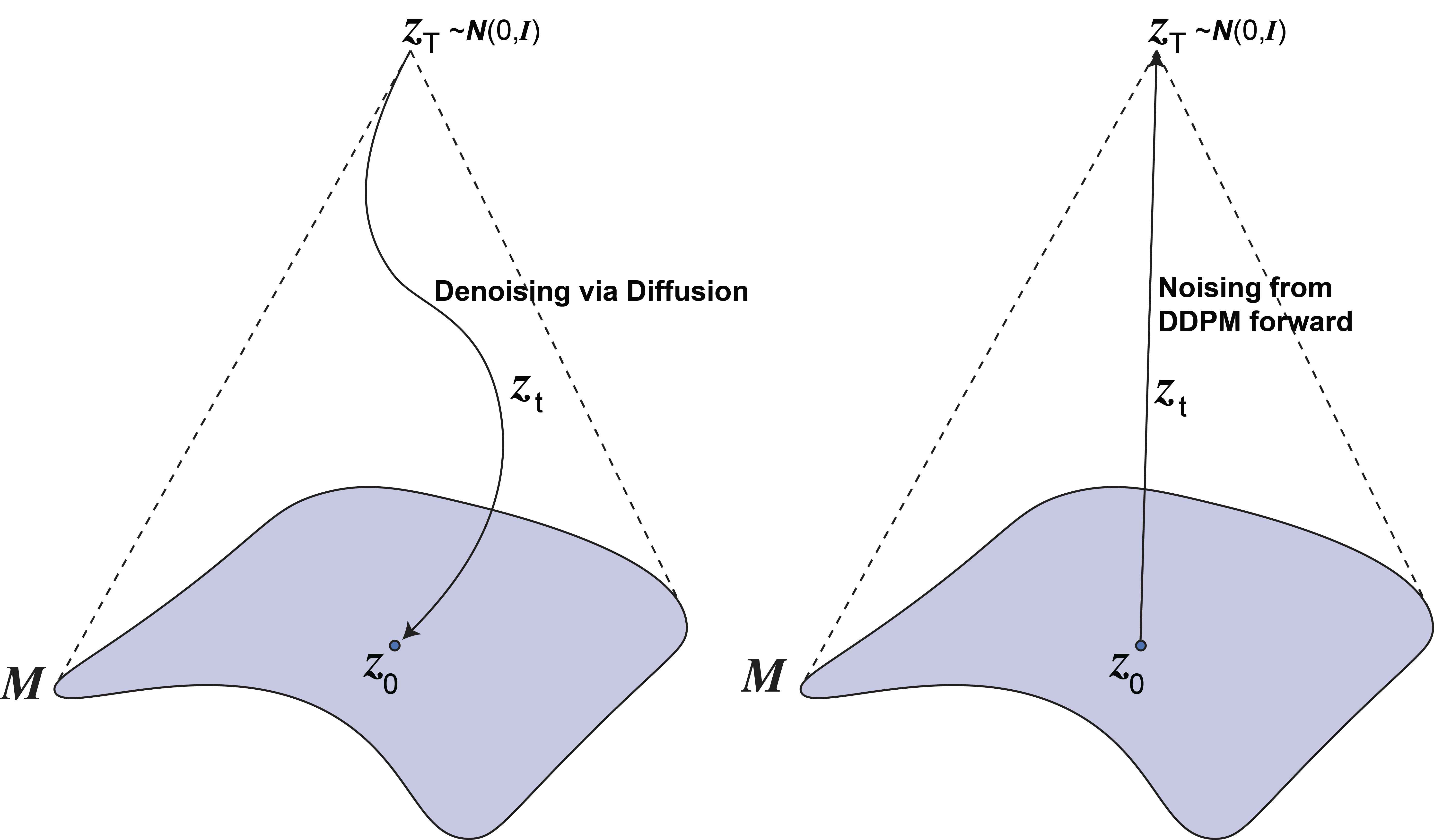
The forward noise process is algorthimic, given here.

$$z_t = \sqrt{\bar{\alpha}_t},z_0 + \sqrt{1-\bar{\alpha}_t},\epsilon, \qquad \epsilon \sim \mathcal{N}(0, I)$$

At train time, the degree/extent of noising is sampled along a number of timesteps between nearly perfect and total corruption between $z_0$ and $z_T$.

We train our model to learn the reverse DDPM process, given here in its $z$ predict form.

$$z_{t-1} = \frac{1}{\sqrt{\alpha_t}} \left( z_t - \frac{1-\alpha_t}{\sqrt{1-\bar{\alpha}_t}},\epsilon_\theta(z_t,t) \right) + \sigma_t z, \qquad z \sim \mathcal{N}(0,I)$$$$\hat{z}_0 = \frac{z_t - \sqrt{1-\bar{\alpha}_t},\epsilon_\theta(z_t,t)} {\sqrt{\bar{\alpha}_t}}$$

I train a model without conditioning to learn how to find the Autoencoder's latent surface and sample from it, sidestepping the question of generative modeling in the VAE by moving it to the latent diffusion model.